Discover the power of the midpoint rule calculator, an indispensable tool that harnesses the midpoint rule for numerical integration. This user-friendly calculator empowers you to effortlessly approximate definite integrals, unlocking a world of possibilities in fields ranging from physics to economics.
The midpoint rule, a versatile numerical integration technique, shines in approximating definite integrals. Its simplicity and effectiveness make it a popular choice, and with our midpoint rule calculator, you can harness its capabilities with just a few clicks.
Midpoint Rule Calculator
Midpoint Rule for Numerical Integration
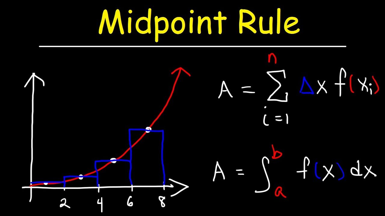
The midpoint rule is a numerical integration technique that approximates the definite integral of a function over an interval. It is based on the idea of dividing the interval into subintervals and approximating the integral over each subinterval using the value of the function at the midpoint of the subinterval.
Example of Using the Midpoint Rule
To approximate the definite integral of the function f(x) = x^2 over the interval [0, 1] using the midpoint rule, we can divide the interval into n subintervals of equal width h = (1-0)/n. The midpoint of each subinterval is then xi = 0 + ih, where i = 1, 2, …, n.
The integral over each subinterval can be approximated by f(xi)
h. The total integral can then be approximated by the sum of the integrals over all the subintervals
“`∫[0,1] x^2 dx ≈ ∑[i=1 to n] f(xi)
h
“`
Applications of the Midpoint Rule
The midpoint rule finds widespread applications in various scientific disciplines, including physics, engineering, and economics, as it provides an efficient means of approximating definite integrals.
In physics, the midpoint rule is commonly used to calculate the area under a curve representing a physical quantity, such as velocity or acceleration. By dividing the time interval into subintervals and approximating the function value at the midpoint of each subinterval, the midpoint rule provides an estimate of the total area under the curve.
Engineering, Midpoint rule calculator
In engineering, the midpoint rule is employed to solve problems involving the calculation of work, energy, and heat transfer. For instance, in thermodynamics, the midpoint rule can be used to approximate the change in internal energy of a system undergoing a process by integrating the specific heat capacity over a temperature range.
Economics
In economics, the midpoint rule is utilized to estimate consumer surplus and producer surplus, which represent the difference between the price consumers are willing to pay and the price they actually pay, and the difference between the price producers receive and the price they are willing to accept, respectively.
By approximating the demand and supply curves using the midpoint rule, economists can determine the equilibrium price and quantity in a market.
Comparison with Other Numerical Integration Methods

The midpoint rule is one of several numerical integration methods used to approximate the definite integral of a function. Other common methods include the trapezoidal rule and Simpson’s rule.The trapezoidal rule approximates the area under a curve by dividing it into trapezoids and summing their areas.
Simpson’s rule uses a parabolic approximation to achieve a higher degree of accuracy.
Advantages and Disadvantages
Midpoint Rule:
- Simple to implement
- Relatively accurate for smooth functions
- Can be used for functions with discontinuities
Trapezoidal Rule:
- Simpler than the midpoint rule
- Less accurate than the midpoint rule for smooth functions
- Not suitable for functions with discontinuities
Simpson’s Rule:
- More accurate than the midpoint rule and trapezoidal rule for smooth functions
- More complex to implement
- Not suitable for functions with discontinuities
Design a Midpoint Rule Calculator
To design a user-friendly midpoint rule calculator, we need to consider the following steps:
User Interface
- Create an input field where users can enter the function to be integrated.
- Include fields for the lower and upper limits of integration.
- Provide a button to initiate the calculation.
- Display the results, including the approximate value of the definite integral and the error estimate, in a clear and concise manner.
Implementation
The calculator can be implemented using a programming language like Python or JavaScript.
The algorithm for the midpoint rule is as follows:
- Divide the interval of integration into n subintervals of equal width.
- Find the midpoint of each subinterval.
- Evaluate the function at each midpoint.
- Multiply each function value by the width of the subinterval.
- Sum the products from step 4 to get the approximate value of the definite integral.
The error estimate for the midpoint rule is given by:
Error estimate = (b-a)^3
f”(c) / 24n^2
where [a, b] is the interval of integration, c is a point in the interval, and n is the number of subintervals.
Example
Let’s consider the function f(x) = x^2 on the interval [0, 1].
Using the midpoint rule with n = 4, we get:
- Subintervals: [0, 0.25], [0.25, 0.5], [0.5, 0.75], [0.75, 1]
- Midpoints: 0.125, 0.375, 0.625, 0.875
- Function values at midpoints: 0.0625, 0.1875, 0.3125, 0.4375
- Approximate value of the definite integral: 0.25
- Error estimate: 0.000694
The exact value of the definite integral is 1/3. Therefore, the midpoint rule provides a good approximation with a small error.
End of Discussion: Midpoint Rule Calculator
The midpoint rule calculator is a valuable asset for students, researchers, and professionals alike. Its intuitive interface and accurate results make it an indispensable tool for solving complex integration problems. Embrace the power of numerical integration today and unlock the full potential of the midpoint rule.