Embark on an intellectual journey with steady state vector calculators, indispensable tools that empower us to decipher the intricacies of complex systems. From the realm of finance to the frontiers of physics, these calculators unravel the secrets of steady state vectors, providing invaluable insights into the behavior of dynamic systems.
Delving into the depths of mathematical modeling, we explore the significance of steady state vectors, uncovering their ability to represent systems in a simplified yet accurate manner. Iterative methods like Jacobi and Gauss-Seidel, along with direct methods such as matrix inversion and QR decomposition, arm us with a diverse arsenal of techniques to calculate these vectors efficiently.
Understanding Steady State Vectors

Steady state vectors are mathematical constructs that represent the long-term behavior of dynamic systems. They are vectors whose components remain constant over time, indicating that the system has reached a state of equilibrium.
Steady state vectors are crucial in mathematical modeling as they provide insights into the asymptotic behavior of systems. They allow researchers to predict the long-term outcomes of complex systems, such as population dynamics, economic models, and engineering systems.
Examples of Systems Represented by Steady State Vectors
- Population Dynamics:Steady state vectors can represent the stable age distribution of a population, indicating the proportion of individuals in each age group over time.
- Economic Models:Steady state vectors can represent the long-term equilibrium levels of economic variables, such as output, consumption, and investment.
- Engineering Systems:Steady state vectors can represent the operating conditions of a system, such as the temperature or pressure of a chemical reactor.
Methods for Calculating Steady State Vectors: Steady State Vector Calculator

Calculating steady state vectors is essential for various applications in fields like linear algebra, Markov chains, and queuing theory. Several methods exist for this purpose, each with its advantages and drawbacks. This content explores the key methods used to calculate steady state vectors, comparing their efficiency and accuracy.
Iterative Methods
Iterative methods are commonly used for calculating steady state vectors due to their simplicity and ease of implementation. These methods involve repeatedly applying a specific update rule to an initial guess until the solution converges to the desired steady state vector.
- Jacobi Method:
The Jacobi method is a basic iterative method where each component of the steady state vector is updated in turn, using the current values of the other components. While straightforward to implement, the Jacobi method can be slow to converge, especially for large systems.
- Gauss-Seidel Method:
The Gauss-Seidel method is an improved version of the Jacobi method that uses the most recently updated values of the components in each iteration. This results in faster convergence compared to the Jacobi method, making it more suitable for large systems.
Direct Methods
Direct methods provide an alternative approach to calculating steady state vectors by directly solving the system of linear equations that defines the steady state. These methods are generally more efficient than iterative methods but require more computational resources.
- Matrix Inversion:
Matrix inversion involves finding the inverse of the coefficient matrix of the linear system. The steady state vector can then be obtained by multiplying the inverse matrix with the constant vector. Matrix inversion is computationally expensive, especially for large systems, but it provides an exact solution if the coefficient matrix is invertible.
- QR Decomposition:
QR decomposition factorizes the coefficient matrix into a product of orthogonal matrices. The steady state vector can be efficiently computed using this factorization. QR decomposition is numerically stable and can handle large systems, making it a preferred choice for many applications.
Comparison of Methods
The choice of method for calculating steady state vectors depends on factors such as the size of the system, the desired accuracy, and the computational resources available. Iterative methods are simpler to implement and require less computational resources, but they may be slower to converge.
Direct methods offer faster convergence and higher accuracy but are more computationally expensive. In practice, QR decomposition is often the preferred choice for large systems due to its efficiency and numerical stability.
Applications of Steady State Vector Calculators
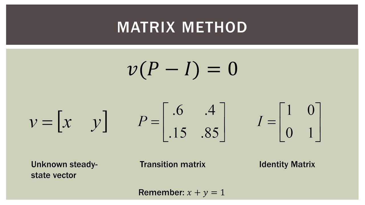
Steady state vector calculators find applications in diverse fields, including finance, physics, and engineering. These calculators provide valuable insights into complex systems by determining the long-term behavior of such systems under specific conditions.
In finance, steady state vector calculators are used to model the long-term behavior of financial markets. By analyzing historical data, these calculators can help investors make informed decisions about asset allocation and risk management. For instance, a steady state vector calculator can determine the long-term expected returns and risks associated with different investment portfolios, allowing investors to optimize their investment strategies.
Engineering
In engineering, steady state vector calculators are employed to analyze the long-term behavior of physical systems. For example, in mechanical engineering, these calculators can be used to determine the steady-state temperature distribution within a complex system, such as a heat exchanger.
This information is crucial for optimizing the system’s performance and ensuring its reliability.
Limitations and Potential Errors
While steady state vector calculators are powerful tools, it is important to be aware of their limitations and potential errors. One limitation is that these calculators assume that the system under consideration is in a steady state, which may not always be the case in real-world applications.
Additionally, these calculators are only as accurate as the data they are based on, so it is important to use high-quality data to obtain reliable results.
Designing a Steady State Vector Calculator
Creating a steady state vector calculator involves defining its features, workflow, and user interface for optimal functionality and ease of use.
Features and Functionality, Steady state vector calculator
A comprehensive steady state vector calculator should offer a range of features, including:
- Ability to calculate steady state vectors for various Markov chains
- Support for both absorbing and non-absorbing chains
- Options for different calculation methods, such as power iteration and Gauss-Seidel iteration
- Provision of detailed results, including the steady state vector and convergence criteria
- Export functionality to save results in various formats
Workflow
The workflow of a steady state vector calculator typically involves the following steps:
- Input the transition matrix of the Markov chain
- Select the desired calculation method
- Execute the calculation
- Review the results
- Export or save the results (optional)
User Interface
The user interface of the calculator should be designed for ease of use, with clear instructions and intuitive navigation. Key considerations include:
- A user-friendly input interface for entering the transition matrix
- Clear labeling and descriptions for all options and parameters
- Visual feedback during the calculation process
- Easily accessible export and save options
Last Word

As we conclude our exploration, we reflect on the transformative impact of steady state vector calculators. They empower us to solve intricate problems, make informed predictions, and gain a deeper understanding of the underlying dynamics of complex systems. However, it is crucial to acknowledge the limitations and potential errors associated with these calculators, ensuring their judicious use.